Drift-Flux vs. Two-Fluid

Marlim3 employs a drift-flux formulation in its transient multiphase-flow solver. In order to better understand the structure, capabilities, and limitations of this formulation, it is useful to compare it with the two-fluid model, which is the most widely used mechanistic framework for transient multiphase pipe flow. OLGA, for instance, is based on this class of model; see Bendiksen et al. (1991).

The purpose of this section is therefore to use the comparison between them to provide physical and mathematical insight into the modeling choices adopted in Marlim3. In particular, the comparison is useful because it clarifies how each formulation distributes transient information among different wave families. For the present documentation, the main goal is to build practical intuition about which variables are mainly associated with fast pressure-carrying waves, which are associated with slower holdup-carrying waves, and what this implies for the numerical treatment adopted later.

Before introducing the governing equations, a brief note on geometry is warranted. In a long pipe, variations of physical quantities in the radial and azimuthal directions are small relative to those in the axial direction, and it is standard practice to work with cross-sectional averages. This collapses the three-dimensional wave problem to a single propagation direction — the pipe axis — giving rise to plane waves, and the one-dimensional formulations that follow rest on this assumption.

Two-fluid model

In a one-dimensional, two-phase two-fluid formulation, two mass conservation equations are employed, one for the liquid phase and one for the gas phase. Likewise, two momentum conservation equations are solved, again one for each phase. Energy conservation may be represented either by a mixture equation or by separate equations for each phase, depending on the desired level of detail.

Focusing first on the two-fluid model, the governing mass and momentum equations can be written as follows.

Liquid mass conservation

\[ A\frac{\partial \left[\rho_l(1-\alpha)\right]}{\partial t} + \frac{\partial \dot{M}_l}{\partial x} = \frac{\Gamma_l}{\Delta L} - \psi \]

Gas mass conservation

\[ A\frac{\partial \left(\rho_g\alpha\right)}{\partial t} + \frac{\partial \dot{M}_g}{\partial x} = \frac{\Gamma_g}{\Delta L} + \psi \]

Liquid momentum conservation

\[ \frac{\partial \dot{M}_l}{\partial t} + \frac{\partial \left(u_l \dot{M}_l\right)}{\partial x} + A(1-\alpha)\frac{\partial p}{\partial x} = - f_{lp}\,\frac{\rho_l U_{ls}^{2}}{2}\,S_w - f_i\,\frac{\rho_m\lvert U_{gs}-U_{ls} \rvert (U_{gs}-U_{ls})}{2}\,S_i + \rho_l g A(1-\alpha)\sin\theta \]

Gas momentum conservation

\[ \frac{\partial \dot{M}_g}{\partial t} + \frac{\partial \left(u_g \dot{M}_g\right)}{\partial x} + A\alpha\frac{\partial p}{\partial x} = - f_{gp}\,\frac{\rho_g U_{gs}^{2}}{2}\,S_w + f_i\,\frac{\rho_m\lvert U_{gs}-U_{ls} \rvert (U_{gs}-U_{ls})}{2}\,S_i + \rho_g g A\alpha\sin\theta \]

Where:

• \(\rho_l\) is the liquid density;
• \(\rho_g\) is the gas density;
• \(\alpha\) is the mixture void fraction;
• \(\psi\) is the interphase mass-transfer term, positive for evaporation and negative for condensation;
• \(\Gamma_l\) is the liquid-phase mass source;
• \(\Gamma_g\) is the gas-phase mass source;
• \(\Delta L\) is the reference length associated with the source terms;
• \(\dot{M}_l\) is the liquid mass flow rate;
• \(\dot{M}_g\) is the gas mass flow rate;
• \(A\) is the pipe cross-sectional area;
• \(S_w\) is the wetted perimeter;
• \(S_i\) is the interfacial perimeter;
• \(U_{ls}\) is the liquid superficial velocity;
• \(U_{gs}\) is the gas superficial velocity;
• \(f_i\) is the interfacial friction factor;
• \(f_{lp}\) is the liquid-wall friction factor;
• \(f_{gp}\) is the gas-wall friction factor;
• \(\theta\) is the pipe inclination angle measured from the horizontal.

In the two-fluid model, each phase is treated in a manner analogous to the corresponding single-phase formulation. However, important distinctions arise once the phases are allowed to interact. Although the void fraction is essential for defining the flow area occupied by each phase, it is not by itself the main quantity responsible for phase coupling. The true hallmark of two-phase flow lies in the interfacial interaction between phases.

Remarkably, among the four equations above, only two terms directly represent the coupling between phases, both of them appearing on the right-hand side. The first, usually of secondary importance, is the interphase mass-transfer term \(\psi\). The second, and generally the dominant coupling mechanism, is the interfacial shear stress term,

\[ f_i\,\frac{\rho_m\lvert U_{gs}-U_{ls} \rvert (U_{gs}-U_{ls})}{2} \]

Special care must therefore be taken in estimating the interfacial friction factor \(f_i\). In one-dimensional two-fluid models, this quantity is not obtained from first principles, but rather from empirical or semi-empirical correlations. Deriving a reliable expression for \(f_i\) is far from trivial, since the forces acting at the interface have a decisive impact on the predictive capability of any two-fluid formulation; see Stuhmiller (1977).

For stratified flow with a smooth interface — the canonical separated-flow configuration — the interfacial closure is comparatively straightforward. In this regime, interfacial friction is essentially associated with film drag rather than form drag. Since form drag depends strongly on interfacial geometry, its absence greatly simplifies closure development. Moreover, because the interfacial shear is relatively small in smooth stratified flow, the coupling between phases is also weak.

By contrast, in wavy stratified flow the interface is disturbed by dispersive waves whose wavelength is much smaller than the pipe diameter, as depicted in the following figure:

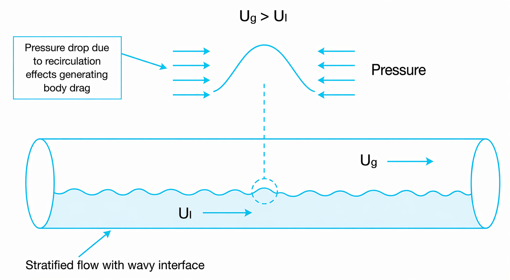
Under these conditions, the interfacial phenomena become substantially more complex and more difficult to model. Even the pressure field in the vicinity of the interface may exhibit highly intricate behavior. In addition, the friction factor is no longer associated solely with film drag: a significant contribution from form drag typically arises, and this contribution is generally much larger than the film-drag component.

As a consequence, the coupling between the liquid and gas phases increases, which is physically expected. In more intuitive terms, strong interfacial drag causes the two phases to move in a more tightly coupled manner, even when the configuration remains clearly separated, as in stratified flow. The same reasoning applies to annular flow, in which the interfacial friction force associated with form drag is also very large, again leading to strong phase coupling.

Defining the interfacial friction factor when form drag plays a relevant role is particularly challenging, because form drag depends strongly on interfacial shape, and this shape may itself be severely distorted by short-wavelength dispersive waves. The difficulty becomes even greater in dispersed-flow configurations. Consider, for example, the canonical dispersed regime, namely dispersed bubbly flow. In that case, constructing a mechanistic or empirical representation of the interfacial processes — including both pressure disturbances at the interface and the corresponding form-drag contribution from a very large number of bubbles — becomes highly nontrivial.

It is therefore reasonable to state that both the degree of phase coupling and the difficulty of modeling interfacial effects follow a hierarchy, ranging from the simplest and most weakly coupled configuration, smooth stratified flow, to highly coupled dispersed configurations such as dispersed bubbly flow.

The objective here is not to present a full characteristic analysis of the two-fluid model represented by the equations above. It suffices to note that such a model gives rise to four families of dynamic waves. For instance, in horizontal stratified flow, the propagation speeds in a two-fluid formulation are approximately given by

\[ c_{1,2} \sim U_g \pm \sqrt{\frac{\partial p}{\partial \rho}} \]

and

\[ c_{3,4} \sim U_l \pm \sqrt{g h} \]

In the expressions above, \(h\) denotes a characteristic liquid-level scale, and the derivative \(\frac{\partial p}{\partial \rho}\) represents an effective gas compressibility contribution, whose precise form depends on the thermodynamic closure adopted.

These four wave families are one of the key mathematical signatures of the two-fluid model. They reflect the fact that the formulation retains separate momentum balances for the two phases.

For subsonic flow, these expressions — even in approximate form — already reveal two wave families with relatively high propagation speeds, primarily associated with gas compressibility, and two slower wave families, closely analogous to gravity waves in open-channel shallow-water models, that is, in the long-wavelength limit relative to the channel height.

Because these are all dynamic waves, every family carries information related to the pressure field. The faster waves do so mainly through gas compression and expansion, whereas the slower waves are associated with variations in liquid level, which modify the mean flow pressure through changes in the hydrostatic liquid head across the pipe cross-section. The actual mechanism is somewhat more involved, but this interpretation captures the dominant effect.

From the standpoint of transient interpretation, this richer wave structure is both an advantage and a burden. It is an advantage because it preserves more of the underlying phase dynamics, especially when fast interfacial and compressibility effects matter. It is a burden because the model then requires more closure detail and a numerical treatment capable of accommodating a wider range of propagation speeds and stronger coupling mechanisms.

The two faster wave families transport pressure information more efficiently. By contrast, the slower waves require comparatively large variations in liquid-film height to produce small pressure changes. Consequently, even when these slower waves are involved in pressure transmission, the most evident system response is generally a variation in void fraction or, equivalently, in liquid holdup. In simplified terms, the faster dynamic-wave pair is more directly associated with the transport of pressure information, whereas the slower dynamic-wave pair is more closely associated with the transport of void-fraction information.

In addition to these dynamic wave families, the source terms appearing in the momentum equations give rise to another class of waves, of lower hierarchy than the dynamic ones: the so-called kinematic waves, or density waves. These waves become important when the inertial terms in the momentum equations are comparatively weak relative to frictional and hydrostatic contributions.

It is important to note that the governing system is not a purely hyperbolic system because of the source terms. As the transient evolves, these source terms may become increasingly influential, and a behavior with elliptic character may emerge. In this regime, pressure can be treated approximately as in a quasi-steady problem, so that the pressure gradient becomes determined essentially by the source terms in the momentum equations.

The principal quantity transported by the kinematic wave is the void fraction. In a two-fluid model, the kinematic-wave propagation speed is approximately given by

\[ c_{\mathrm{kin}} \sim \frac{\partial U_{sg}}{\partial \alpha} \]

This value is also often close to the gas velocity itself. This is an important result: whenever the dynamic terms become of secondary relevance, the kinematic wave assumes most of the responsibility for transporting void-fraction information.

In a drift-flux model, a kinematic wave does not arise as directly as in the two-fluid formulation. Nevertheless, the slowest dynamic wave family in the drift-flux model is itself closely related to the mean gas velocity. In this sense, the two approaches become similar with respect to the transport of void-fraction information in two-phase flow.

Consider the initial condition illustrated in the next figure: a pipe divided into two regions by a ball valve.

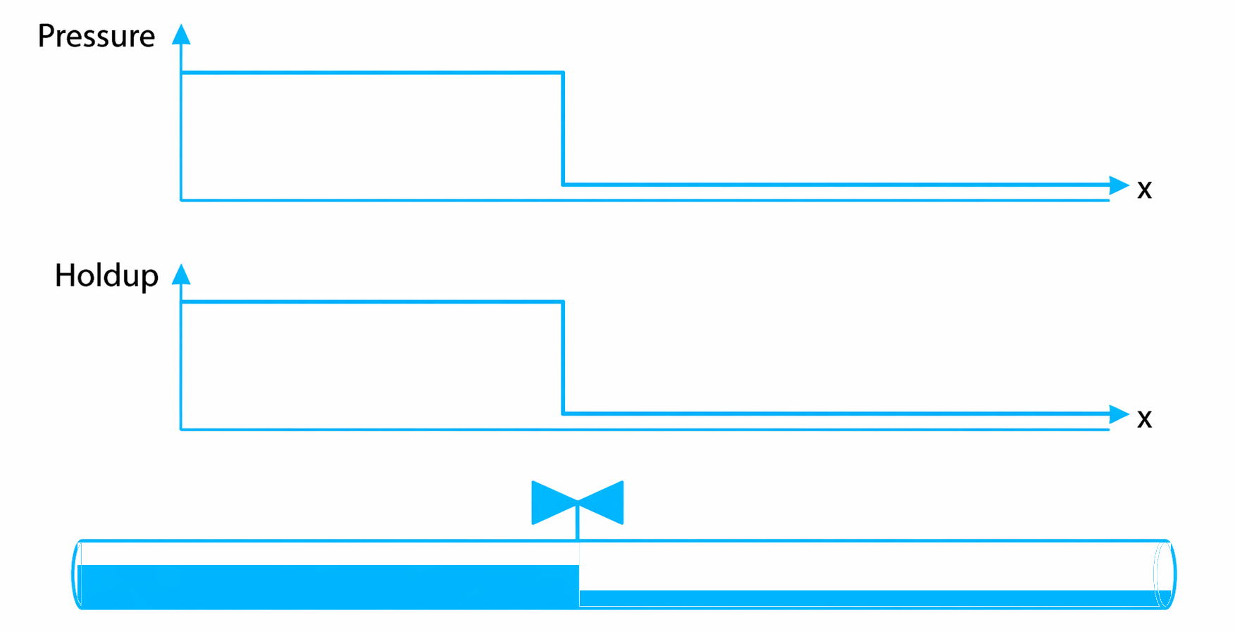
If the valve is opened rapidly, the system undergoes fast transient changes, partly governed by the faster wave families and partly governed by the slower ones.

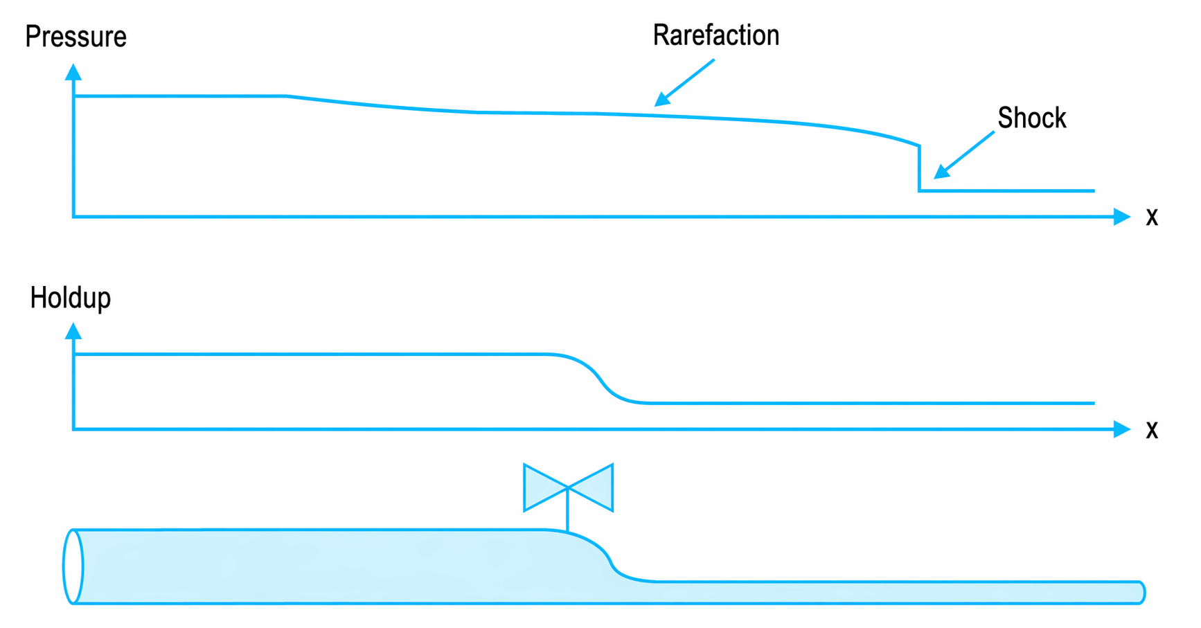
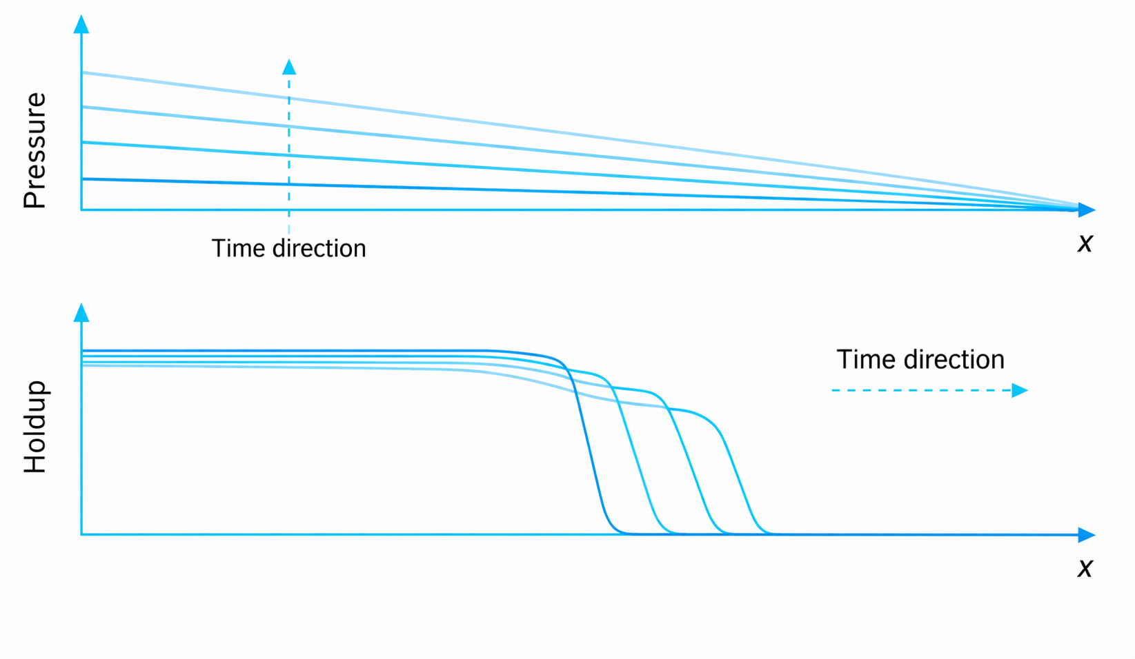
As expected, pressure information propagates more rapidly than holdup information. The latter is associated with the slower dynamic waves and, once dynamic effects related to fluid acceleration become negligible, the transient behavior is governed predominantly by the kinematic wave, also referred to as the continuity wave or density wave; see Wallis (1969).

The following figure illustrates the holdup information propagation process, when hyperbolic phenomena related to the physical quantity of pressure become of little relevance.

Drift-flux model

As discussed above, the principal difficulty of the two-fluid model lies in the reliable representation of interfacial effects. The drift-flux model emerges as a simplification of the two-fluid formulation and seeks to bypass, at least partially, the need for a detailed description of interfacial effects in multiphase flow. The classical reference for this model is Zuber and Findlay (1965).

The main structural difference relative to the two-fluid model is the reduction in the number of momentum equations. Instead of solving one momentum equation for each phase, the drift-flux model employs a single mixture momentum equation:

Liquid mass conservation

\[ A\frac{\partial \left[\rho_l(1-\alpha)\right]}{\partial t} + \frac{\partial \dot{M}_l}{\partial x} = \frac{\Gamma_l}{\Delta L} - \psi \]

Gas mass conservation

\[ A\frac{\partial \left(\rho_g\alpha\right)}{\partial t} + \frac{\partial \dot{M}_g}{\partial x} = \frac{\Gamma_g}{\Delta L} + \psi \]

Mixture momentum conservation

\[ \frac{\partial \dot{M}_m}{\partial t} + \frac{\partial \left(u_l \dot{M}_l + u_g \dot{M}_g\right)}{\partial x} + A\frac{\partial p}{\partial x} = f_m\,\frac{\rho_m j^2}{2}\,S_w + \rho_m g A\sin\theta \]

Compared with the two-fluid model, the drift-flux formulation replaces the two separate phase-momentum equations by a single mixture momentum balance. This reduction simplifies the mathematical structure of the model and removes the explicit interfacial shear term from the momentum equations.

The main consequence of this reduction is that the terms associated with interfacial forces — interfacial drag and local pressure disturbances at the interface — become embedded in the model rather than appearing explicitly. Naturally, the formulation now requires an additional constitutive relation so that it can be closed mathematically and still represent, in physical terms, the coupling between phases. Although the interfacial terms are hidden, the coupling still occurs at the interface. Therefore, any constitutive relation introduced in the drift-flux framework must ultimately be derived from the physical processes taking place there.

An instructive way to motivate such a constitutive relation is through a simple experiment. Consider a single bubble rising in a liquid. If the bubble ascends at constant velocity, the net force acting on it must be zero. One of the forces is buoyancy; the other is the resultant of the forces acting at the interface, essentially film drag and form drag. The bubble translational velocity, denoted here by \(U_t\), is therefore a direct consequence of the force balance, part of which originates from interfacial effects.

In this sense, analyzing the translational velocity of one phase relative to the surrounding fluid provides an indirect, or hidden, representation of the interfacial forces responsible for phase coupling. If the surrounding medium moves with velocity \(j\), the bubble velocity may be written simply as

\[ U_{\mathrm{bubble}} = j + U_t \]

The main advantage of models based on relative velocities between phases is that they are much easier to obtain experimentally and to represent empirically than models attempting to resolve localized pressure disturbances at the interface directly. Of course, relations written specifically for the rise velocity of a single bubble are not directly suitable as a general closure for two-phase pipe flow, but they indicate the appropriate modeling strategy.

One cannot, for example, immediately extrapolate the previous expression to a relation such as \(U_g = j + U_t\), with \(j\) interpreted as the mixture velocity, without further averaging considerations. Consider dispersed bubbly flow in a pipe. The problem is now more complex than that of a single bubble rising in a quiescent liquid, because the gas velocity must be represented in an averaged sense over the pipe cross-section. Since the local mixture velocity varies across the cross-section, an averaging procedure is required to obtain a representative gas velocity relative to the mixture. To account for this nonuniformity, the distribution parameter is introduced; see Ishii and Hibiki (2006):

\[ C_0 = \frac{\langle \alpha_g j \rangle}{\langle \alpha_g \rangle \langle j \rangle} \]

where \(\langle \cdot \rangle\) denotes cross-sectional averaging. With this definition, one may write a more general kinematic relation connecting gas velocity to mixture velocity:

\[ U_g = C_0 j + U_d \]

where \(U_d\) is the drift velocity. The value of \(C_0\) depends on how the gas fraction is distributed over the pipe cross-section and on the velocity profile of the mixture. When gas is distributed nearly uniformly over the cross-section, \(C_0\) tends to be close to 1, as in annular flow. In turbulent flow, when gas is concentrated near the pipe center, \(C_0\) tends to approach the multiplier associated with the maximum velocity of the turbulent profile, typically about \(1.2\). This behavior is observed, for instance, in the translational velocity of the nose of an elongated bubble or Taylor bubble. In laminar flow, by contrast, \(C_0\) may approach 2.

For mixture velocities of order unity or greater, the drift velocity tends to play a secondary role, whereas the distribution parameter becomes more relevant. In segregation-dominated processes — especially those of interest in shut-in analyses or severe slugging — the drift velocity becomes increasingly important.

The key point is that a wide range of drift-flux correlations is now available for different flow configurations. It is true that such correlations are usually derived from steady-state experiments, which may limit their applicability to transient problems. However, this limitation does not appear to be critical for slow transients. Furthermore, because only the mixture momentum equation is retained, the drift-flux model is often regarded as particularly suitable for flow patterns with strong phase coupling; see Ishii and Hibiki (2006). This includes dispersed bubbly flow, slug flow, and, in some cases, annular flow when flooding is absent. More recently, broad drift-flux correlations have been proposed that cover a wide variety of flow situations, including segregation processes; see Bhagwat and Ghajar (2014).

Regarding wave propagation, the isothermal drift-flux model exhibits three wave families. Two of them, as usual, are primarily associated with gas compressibility. The third is a low-speed dynamic wave whose propagation speed is approximately equal to the mean gas velocity. This third family is especially relevant in the drift-flux model for most transient problems of interest in production and transport systems, since it is the wave family chiefly responsible for transporting void-fraction information. For a complete eigenvalue analysis of the one-dimensional isothermal drift-flux model, see Santin and Rosa (2016).

This reduction from four dynamic families in the two-fluid model to three in the drift-flux model helps explain why the latter is attractive for the class of problems targeted by Marlim3. The formulation gives up part of the detailed phase-wise dynamic description, but it preserves the transport mechanism that is most important for slow production-system transients: the comparatively slow propagation of gas fraction and liquid holdup. At the same time, the fast pressure-related families remain present through the compressible mixture description, which is why the later numerical treatment still solves pressure implicitly. In short, the drift-flux model may be viewed here as a deliberate compromise: it is simpler than a full two-fluid model, but it still retains the wave structure needed to represent the dominant transient mechanisms in the intended applications.

The next section presents the derivation of the model adopted in the Marlim3 transient solver.

References

Bendiksen, K. at al, (1991), The Dynamic Two-Fluid Model OLGA: Theory and Application, SPE Prod Eng 6 (02), pp 171-180;

Bhagwat, S. & Ghajar, A., (2014), A flow pattern independent drift flux model based void fraction correlation for a wide range of gas–liquid two phase flow, International Journal of Multiphase Flow Volume 59, February 2014, pp 186-205;

Ishii, M. & Hibiki, T. (2006), Thermo-fluid Dynamic of Two-Phase Flow, Springer;

Santim, C. Rosa, E., (2015); Roe-type Riemann solver for gas-liquid flows using drift flux model with an approximate form of the Jacobian matrix, Numerical Methods in Fluids, Volume 80, issue 9;

Stuhmiller, J., H., (1977), The Influence of Interfacial Pressure Forces on the Character of Two-Phase Flow Model Equations; International Journal of Multiphase Flow, Vol 3, pp. 551-560;

Wallis, G.B., (1969); One-Dimensional Two-Phase Flow; McGraw-Hill.

Zuber, N. and Findlay, J.A. (1965) Average Volumetric Concentration in Two-Phase Flow Systems. Journal of Heat Transfer, 87, pp 453-468.