Comparison of horizontal and vertical multiphase flows
Marlim3 - Python Tutorials
In this notebook, two base cases in steady state are set up (horizontal and vertical) and, from them, some system parameters are varied to analyze the behavior of multiphase flow curves in each situation.
The examples are inspired by Section 5.5 of ANDREOLLI (2016).
%load_ext autoreload
%autoreload 2

import numpy as np
import marlim3
import copy
Introduction
One of the main areas of focus in the discipline of flow assurance is the modeling and simulation of the flow process of produced fluids from the wellbore bottom to the surface platform, passing through subsea lines. Modeling this process is fundamental, for example, to quantify the energy loss of the fluid along the pipeline, which may generate the need for artificial lift methods, such as gas-lift or subsea pumping. Additionally, heat exchange between the fluid and the pipeline surroundings can influence processes such as hydrate and wax formation.
In general, the three most relevant properties to observe during a flow simulation are: pressure, temperature, and liquid holdup (fraction of the pipe's cross-section occupied by liquid). One factor that exerts great influence is the slip between phases, caused by the velocity difference between them, which contributes to energy losses in the flow.
An important aspect of oil flow is the presence of multiple phases together, which characterizes the flow as multiphase. In these cases, various phase arrangements, or flow patterns, can emerge at different points in the pipeline, depending mainly on the flow rates of each phase. Below, we present a representation of the most commonly observed arrangements:
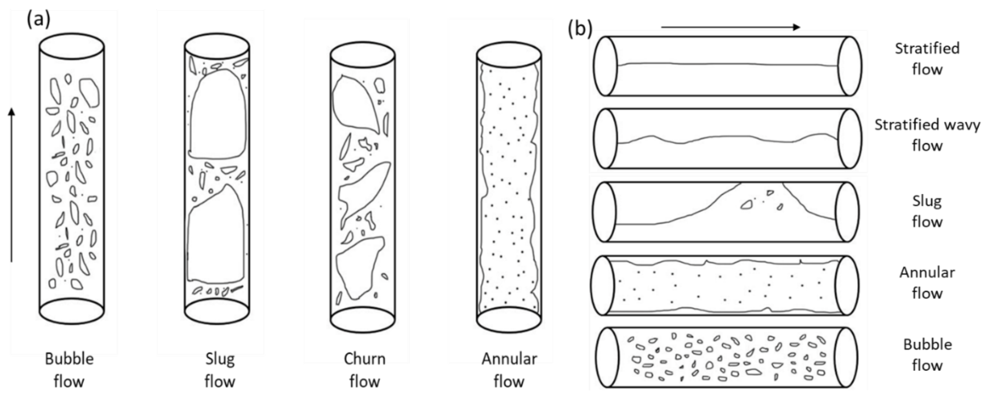
- Bubble: characterized by the presence of small gas bubbles dispersed in the liquid. The holdup is high. In the vertical case, it occurs both at low liquid flow rates (with slip between phases) and at high liquid flow rates (in this case, bubbles disperse in the liquid without significant slip). In the horizontal case, this arrangement manifests only at high liquid flow rates.
- Slug: arrangement in which large gas bubbles form and move regularly through the liquid.
- Churn: present only in the vertical case, it characterizes a transition between slug and the next arrangement, annular, as gas flow rate increases.
- Annular: arrangement in which gas flows through the center of the pipeline, while liquid forms a film on the wall. Occurs at high gas flow rates.
- Stratified: present only in the horizontal case, characterized by gravitational separation between gas and liquid. Occurs at low liquid and gas flow rates. With increasing gas flow rate, the interface between phases may present waves, resulting in a wavy stratified arrangement.
In the video below, you can see an interesting visualization of phase arrangements in a vertical pipeline (plus a pretty cool soundtrack):
from IPython.display import YouTubeVideo
YouTubeVideo("pkhVxqDg_fk")
In this tutorial, we will use Marlim3, Petrobras' most advanced internal multiphase flow simulator, developed at CENPES, to understand how the coexistence of liquid and gas phases introduces important distinctions in flow behavior in horizontal and vertical pipelines. Marlim3 allows simulations in two types of regimes:
- Steady state regime, in which flow conditions such as pressure, temperature, and liquid holdup are considered constant over time, reflecting a stationary state of the system.
- Transient regime, which takes into account the evolution of these conditions over time, allowing the analysis of dynamic events such as flow rate variations or valve openings.
In this notebook, we will focus exclusively on steady state simulations.
Base case setup
We will populate a Branch object from Marlim3 for the horizontal case:
base_case_horizontal = marlim3.Branch()
The vertical case will be created later from a copy of the horizontal case.
fluid = {
    "id": 0,
    "api": 32,
    "gor": 100,
    "gasDensity": 0.7,
    "bsw": 0.0,
}

base_case_horizontal.productionFluid = [fluid]
Marlim3 offers other fluid modeling possibilities: flash tables and compositional models.
Line material
The material used will be steel:
steel = {
    "id": 0,
    "type": 0, # solid
    "conductivity": 58, #W/m.K
    "specificHeat": 480, #J/kg.K
    "rho": 7850, #kg/m3
}

base_case_horizontal.material = [steel]
Cross-section
We will define a cross-section whose wall contains a single layer.
The layer, with $1$" thickness, will be made of material with ID = 0 (steel).
The cross-section will have a $10$" internal diameter and $0.183$ mm absolute roughness.
layer = {
    "materialId": 0, # id of the material defined earlier
    "layerMeasurementType": "THICKNESS",
    "thickness": 0.0254, #m
}

cross_section = {
    "id": 0,
    "innerDiameter": 10*0.0254, #m
    "roughness": 0.183e-3, #m
    "layers": [layer]
}

base_case_horizontal.crossSection = [cross_section]
Duct
The duct will be $2500$ m long and will be divided into $20$ discretization cells.
The external environment will be the atmosphere and environmental conditions will be defined at the beginning and end of the pipeline (relative lengths $0$ and $1$, as specified in the measuredPosition field). At intermediate points, values are obtained by linear interpolation.
We will use the previously defined cross-section (crossSectionId = 0).
The angle will be $0$, as we are setting up the horizontal base case.
n_cells = 20

total_length = 2500 #m

segment = {
    "numCells": n_cells,
    "length": total_length/n_cells #m
}

ambient_conditions = {
          "measuredPosition": [0, 1],
          "ambientTemp": [40, 20], #degC
          "ambientVel": [0.5, 0.5], #m/s
}

duct = {
        "id": 0,
        "crossSectionId": 0, # id of the cross-section defined earlier
        "environment": 2, # atmosphere
        "angle": 0, #rad
        "discretization": [segment],
        "initialConditions": ambient_conditions
}

base_case_horizontal.productionPipe = [duct]
If there were variations in pipeline properties, more ducts could be incorporated into the productionPipe list and the resulting pipeline would be composed of the sequence of ducts in the list.
After defining the ducts, we can visualize the geometry:
base_case_horizontal.plot_geometry();
It is, indeed, a simple horizontal pipeline.
Boundary conditions
The boundary conditions (BC) in our case are $1$) liquid flow rate upstream and $2$) pressure downstream.
BC $1$ must be defined through a liquid source placed right at the beginning of the pipeline (in the case below, $0.1$ m measured length).
upstream_bc = {
    "id": 0,
    "prodFluidId": 0, # id of the fluid defined earlier
    "measuredLength": 0.1, #m
    "time": [0], #s
    "liquidFlowRate": [1500], #sm3/d
    "temperature": [40] #degC
}

base_case_horizontal.liquidSource = [upstream_bc]
BC $2$ must be defined through the separator field.
downstream_bc = {
    "time": [0], #s
    "pressure": [2], #kgf/cm2
}

base_case_horizontal.separator = downstream_bc
Simulation output specification
We can choose which output variables (in our case, profiles, or variations along the line) will be reported as simulation results.
Below, we specify pressure, temperature, liquid holdup, flow pattern arrangement, and friction and hydrostatic components of pressure drop.
output_vars_list = ["pressure",
                    "temperature",
                    "holdup",
                    "flowPattern",
                    "frictionPressureGradient",
                    "hydrostaticPressureGradient"]

output_vars = {"time": [0]} | {var: True for var in output_vars_list}

base_case_horizontal.productionProfile = output_vars
With the horizontal base case ready, we can now copy it and change the angle to create the vertical base case:
base_case_vertical = copy.deepcopy(base_case_horizontal)
base_case_vertical.productionPipe[0]['angle'] = np.pi/2
base_case_vertical.plot_geometry();
Running simulations and analyzing results
Varying flow rate
In the cell below, we specify four flow rates and simulate the vertical and horizontal cases for each one:
#%%time

flow_rates = [200, 2000, 4000, 6000]

cases_v = []
cases_h = []

for flow_rate in flow_rates:

    cases_h.append(copy.deepcopy(base_case_horizontal))
    cases_h[-1].liquidSource[0]['liquidFlowRate'] = [flow_rate]
    cases_h[-1].simulate()

    cases_v.append(copy.deepcopy(base_case_vertical))
    cases_v[-1].liquidSource[0]['liquidFlowRate'] = [flow_rate]
    cases_v[-1].simulate()
*******************************************************************************
                                  UFA!!!!!!!!
                  Uma jornada de mil quilometros come�a com um unico passo
    Lao-Tse tomando coragem para simular um caso de parafinacao em dutos de producao
*******************************************************************************
ARQUIVO DE LOG: simulacao.log

*******************************************************************************
                                  UFA!!!!!!!!
                        Quem vive de navegar, o vento e quem lhe comanda
                          Seu Pereira na feira de artesanatos numericos
*******************************************************************************
ARQUIVO DE LOG: simulacao.log

*******************************************************************************
                                  UFA!!!!!!!!
                          Post Coitum Omine Animal Triste Est
                         Galeno de Pergamo do Transiente Longo
*******************************************************************************
ARQUIVO DE LOG: simulacao.log

*******************************************************************************
                                  UFA!!!!!!!!
                  A necessidade e a mae da inovacao, mas a paciencia e o pai
                                      Marcao da Oficina
*******************************************************************************
ARQUIVO DE LOG: simulacao.log

*******************************************************************************
                                  UFA!!!!!!!!
           'Ouca-me. O fim quase nunca esta longe, em nenhum momento!'
                     J. California Cooper depois da simulacao divergir
*******************************************************************************
ARQUIVO DE LOG: simulacao.log

*******************************************************************************
                                  UFA!!!!!!!!
O sucesso nao e uma linha reta, e um jogo de resistencia, e cada tropeco e apenas um degrau a mais para a vitoria!
                                    Mario Pascal do Insta
*******************************************************************************
ARQUIVO DE LOG: simulacao.log

*******************************************************************************
                                  UFA!!!!!!!!
                   Infeliz e o espirito ansioso pelo futuro.
                              Seneca do Mindfulness
*******************************************************************************
ARQUIVO DE LOG: simulacao.log

*******************************************************************************
                                  UFA!!!!!!!!
                        Quem vive de navegar, o vento e quem lhe comanda
                          Seu Pereira na feira de artesanatos numericos
*******************************************************************************
ARQUIVO DE LOG: simulacao.log
Phew!! Eight simulations were executed. To visualize the results, we can create two Scenarios type objects in Marlim3, providing each of them with a dictionary containing the cases, in the pattern {'case legend': 'case object'}:
scenarios_h = marlim3.Scenarios({f'Q = {flow_rate} sm3/d': cases_h[i] for i, flow_rate in enumerate(flow_rates)})
scenarios_v = marlim3.Scenarios({f'Q = {flow_rate} sm3/d': cases_v[i] for i, flow_rate in enumerate(flow_rates)})
Horizontal cases
scenarios_h.plot_profiles(line='production');

Vertical cases
scenarios_v.plot_profiles();

If this is your first contact with this type of results, analyze them and take some time to think about them before reading the explanations below!!
- Horizontal case
- Pressure: the higher the flow rate, the higher the upstream pressure associated with the downstream boundary condition pressure. In other words, the greater the pressure difference and therefore the greater the pressure drop. This is due to greater energy loss in the flow due to friction phenomenon when fluids flow with higher velocity.
- Temperature: the higher the flow rate, the higher the arrival temperature, because an increase in fluid mass results in greater thermal capacity, resulting in less temperature decrease.
- Holdup: the higher the flow rate, the higher the resulting upstream pressure and the fluid under this condition has less free gas, so the holdup is higher. As the fluid flows, pressure drops and gas is gradually released, decreasing the holdup. For very low flow rate cases, such as $200$ sm$^3$/d, the holdup is practically constant because the pressure variation is very low.
- Flow pattern: at very low flow rates, such as $200$ sm$^3$/d, the flow is stratified (-1). Higher flow rates result in greater liquid entrainment and therefore arrangements such as annular (-2), churn (-2), or slug (2).
- Hydrostatic term of pressure drop: since the pipeline is horizontal, there is no resistance from gravity to the flow and therefore there is no hydrostatic term in the pressure drop.
- Friction term of pressure drop: the higher the flow rate, the higher the flow velocities and therefore the more the fluid loses energy due to friction phenomenon.
In the vertical case, there is a balance between the friction and hydrostatic components of pressure drop, leading to different behaviors from horizontal flow.
- Vertical case
- Pressure: analyzing only the three curves with higher flow rates, the behavior is similar to the horizontal case. However, notice that the lowest flow rate of $200$ sm$^3$/d corresponds to the highest pressure drop! This occurs because in this case the flow rate is so low that the gas cannot carry the liquid, which accumulates in the column, greatly increasing the holdup and consequently also the hydrostatic pressure drop, as verified in the other graphs.
- Temperature: the trend is similar to the horizontal case, but the curves for the various flow rates are closer. As the pressure drop is high, there is a large variation in holdup and the dominant mechanism for temperature decrease is no longer heat exchange with the environment but rather gas expansion (Joule-Thompson effect); hence, the lower sensitivity to flow rate.
- Holdup: the initial holdups are higher than in the horizontal case, since the resulting upstream pressures are higher. To understand the trend inversion in the very low flow rate case, see the first item (pressure).
- Flow pattern: for the lowest flow rate, the predominant arrangement is bubble (1), with higher holdup. For the highest flow rates, the slug arrangement predominates (2).
- Hydrostatic term of pressure drop: the hydrostatic term of pressure drop now exists, since the flow must overcome the force of gravity to occur. To understand the trend inversion in the very low flow rate case, see the first item (pressure).
- Friction term of pressure drop: the behavior is practically the same as in the horizontal case, but with lower values, since the flow velocities are lower in the vertical case. This occurs because, in the vertical case, the flow presents higher holdups for the same mass flow rate; therefore, the specific volume of the mixture is lower, decreasing the volumetric flow rate and consequently the velocity.
Try it yourself!
1. Repeat the previous analyses using more profile variables in the output for visualization. For example, visualize the local flow velocities of gas and liquid to verify the relationships with the friction term of pressure drop and holdup mentioned earlier. Consult the JSON Schema available in the Marlim3 repository to learn about the possible output variables that can compose the profiles.
2. Using $1500$ sm$^3$/d as the inlet flow rate, run new simulations varying the following properties:
- Line diameter ($5$" to $20$");
- Gas-oil ratio, GOR ($0$ to $2000$ Sm$^3$/Sm$^3$, with more simulations in the initial range);
- Oil density, API ($15$ to $25$°).
What do you expect the behavior of pressure drop to be in each case? In which ones do you think there will be a trend inversion due to the balance between hydrostatic and friction in vertical flow?
3. Add one more layer to the pipeline's cross-section, with insulating characteristics. What are the effects on the temperature profiles in each case?